Lizard Classification (Deep Learning Challenge)
Context
This was a group project for the Artificial Intelligence course in my second year at Thomas More, run as a Kaggle competition. The three of us (Yorben, Warre and myself) had to build a deep learning model that could tell apart 7 lizard species from photos: black spiny-tailed iguana, brown anole, Cuban knight anole, desert iguana, green anole, green iguana and Lesser Antillean iguana. The catch was that several of these look nearly identical, and we only had 1,334 training images (around 190 per class). So it was a small, fine-grained image classification problem where overfitting was the real enemy.
What we built
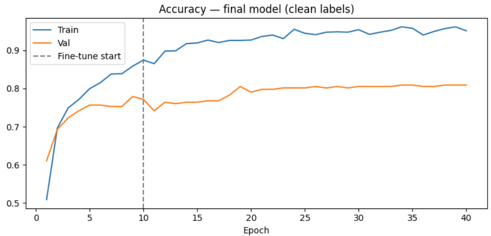
An image classifier that reaches about 79% validation accuracy and scored 0.831 on the Kaggle leaderboard. It runs on EfficientNetV2S with transfer learning, trained in two phases, with a full pipeline around it: exploratory analysis, augmentation, automatic label-noise correction, and test-time augmentation at inference. Everything lives in one documented notebook where each choice is explained, not just coded.
Why we made it
The goal was to get real experience with the modern deep learning workflow instead of calling .fit() once and hoping for the best. We wanted to see how far we could push a small dataset with the right techniques, and to understand why each step actually helped. The competition format kept us honest: every idea had to move the leaderboard, not just sound clever.
How we made it
We started with EDA and confirmed the classes were roughly balanced, then made an 80/20 stratified split so both sets kept the same class ratios. Because the dataset was small, we added mild augmentation (horizontal flip, small rotation, zoom and contrast) at 384×384, which is EfficientNetV2S's native resolution. We deliberately kept it gentle so fine details like scale patterns and dewlap colour weren't washed out.
For the model we first tried ResNet50, which stalled around 67% on Kaggle, then switched to EfficientNetV2S pretrained on ImageNet, which did clearly better on this fine-grained task. Training happened in two phases: first head-only with the backbone frozen (learning rate 1e-3), then fine-tuning the top blocks (layers 400 to 513) at a much lower rate (1e-5) with a cosine decay schedule, keeping all BatchNorm layers frozen so their statistics wouldn't drift on such a small set. Dropout (0.4), label smoothing (0.1) and early stopping kept overfitting under control.
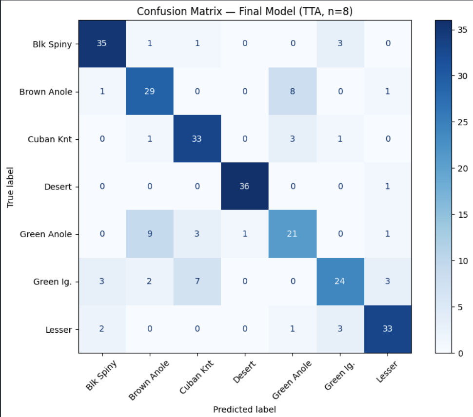
Two extra steps gave us most of the final gains. We used the trained model to flag likely mislabeled images (confident predictions that disagreed with the given label), auto-corrected the ones above 90% confidence, and retrained from scratch on the cleaned labels. Then at inference we applied test-time augmentation, averaging predictions over several augmented views of each image, which works like a free ensemble and helps most on the ambiguous green species.
What we used
- Python with TensorFlow and Keras for the model and training loop
- EfficientNetV2S (ImageNet pretrained) as the backbone, with two-phase transfer learning
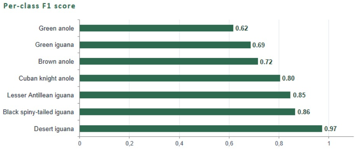
- scikit-learn for the stratified split and evaluation (confusion matrix, per-class F1)
- pandas, numpy and matplotlib for data handling and EDA
- Kaggle for the competition and leaderboard scoring
- AI tools used transparently: Claude Code for writing and debugging, Perplexity and Gemini for researching and explaining techniques. We verified and adapted everything ourselves.
My contribution
We worked as a loop rather than splitting the project into silos. Each of us went off and tried our own ideas independently (different architectures, augmentation settings and training tricks), then came back together to compare what actually worked and merge the best parts into the shared notebook. A lot of the final result came from that back and forth: someone's experiment would beat the current best, we'd fold it in, and the baseline would climb again. I brought my own experiments into that cycle and helped pull our findings together into the version we submitted.
Key takeaways
- On a small dataset, technique beats raw model size. The climb from 67% to 83% came less from a bigger network and more from label cleaning, sensible augmentation and TTA.
- Data quality is worth chasing. Finding and fixing a handful of wrong labels gave one of the single biggest jumps in accuracy.
- The confusion matrix tells you where to look. It showed the model mostly struggled with the visually similar green anoles and iguanas, which is exactly where more data would help next.
- A tight team experiment loop, everyone trying things and pooling the best, got us further than dividing the work into separate parts would have.